

How To Use Excel Chart Templates 2021
So, you're looking for a way to create a Gantt chart that will blow everyone away, simply all the searching you've done online leads you to this mediocre graph?
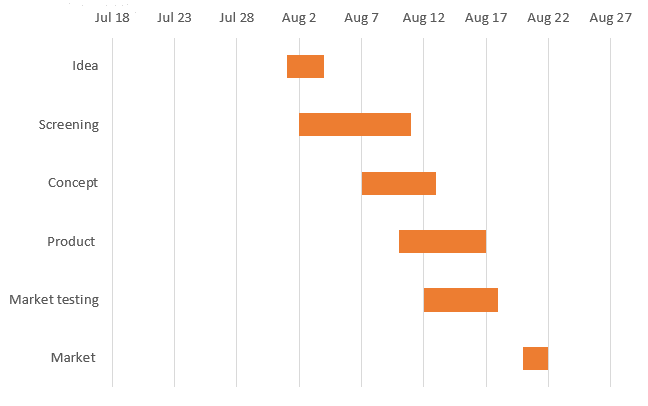
Let'southward be honest. It'south 2021, and this chart simply doesn't cutting information technology as a projection management tool that you would actually use. But are there any alternatives? Well, yous've come to the right place!
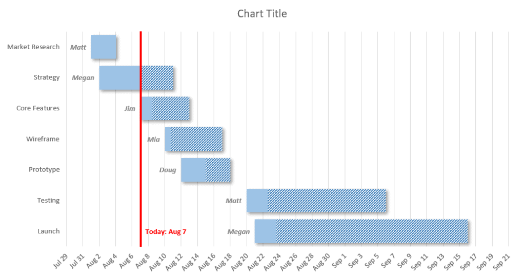
In this step-by-stride tutorial, you will learn how to create this professional-looking Gantt chart in Excel without any add-ons—fifty-fifty if you're a complete newbie:
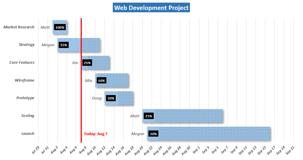
The beauty of this Excel Gantt chart is that information technology supports a whole bunch of critically of import features that third-party software providers typically charge yous for:
- Unlimited tasks
- Total customization
- The electric current date line
- Tracking the progress on each task
- Assignees
- Sleek design
With this Gantt chart, you are in the driver'due south seat. You take total command over every single element of the graph. You lot can even utilise it in your dashboards, as opposed to in-cell Gantt charts. And you tin can become all of that (and more) without paying a dime.
The setup process is a chip lengthy and may take you anywhere betwixt 10 and 15 minutes. But the payoff is tremendous.
Nosotros have broken everything downwards into pocket-sized, simple steps to make sure y'all tin can really build out the same Gantt chart illustrated above on your own. Without beating around the bush, let's leap right in—we've got some charting to do!
Also, if you're short on time, you can grab a Gantt chart template and follow the setup instructions nosotros mapped out at the end of the article. The template is completely free and you don't have to give away your electronic mail accost or sign upwardly for anything to get information technology.
Also, check out our superlative picks for the all-time Gantt chart software if y'all're looking to take your project direction to the side by side level.
Step 1. Add together the Project Data
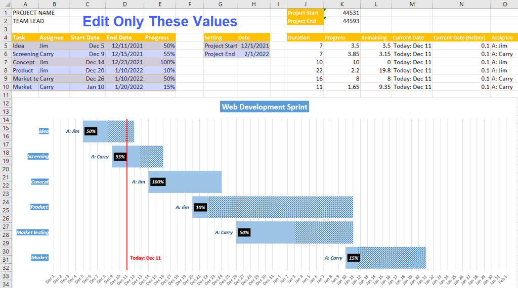
Start with calculation all the actual project data using the screenshot beneath:
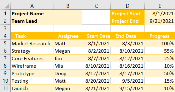
Hither's the breakdown of the tables to help you arrange it to your ain specifications:
- Projection Name & Team Lead – These two cells won't exist used in the setup procedure and serve merely to provide your users with more context.
- Projection Start & Project End – These 2 dates define the offset and end of your project and volition be used for charting the horizontal axis of your Gantt chart.
- Task – These values determine the actual tasks and will be charted as vertical centrality values.
- Assignee – These are going to exist used only as data labels. Alternatively, you tin can use the departments responsible for the execution of a given job.
- Beginning Date & End Date – These columns ascertain the beginning and end of each chore. Enter the dates in the dd/mm/yyyy format.
- Progress – This column indicates the task completion stage. If y'all don't want to use this feature, set all the values to 100% and alter the background and font color to white to hide the cavalcade.
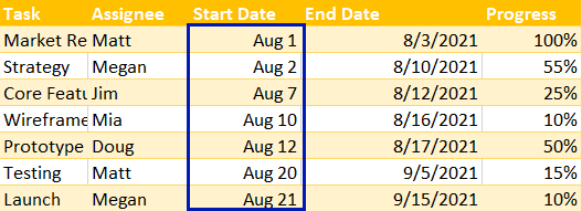
Right out of the gate, we need to format the dates in column Start Date in a dissimilar way and then the horizontal axis will display corking-looking dates.
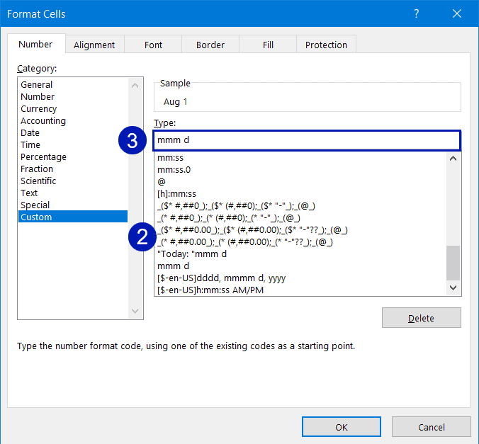
1. Highlight the values in column Outset Date (C5:C11), right-click, and select "Format Cells."
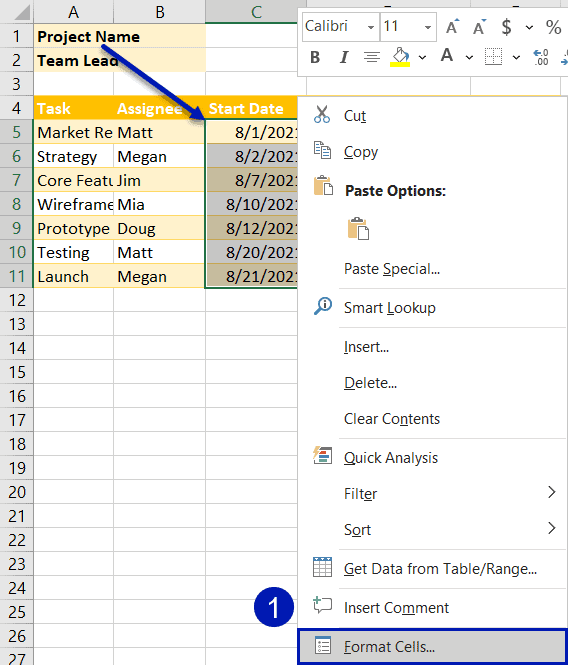
2. In the Format Cells dialog box, under "Category," choose "Custom."
3. In the "Type" field, enter mmm d to ready a custom date format that will make it a lot easier to read the chart.
One time there, hither's how the dates you modified should await:
Step 2. Prepare the Chart Data
Since our Gantt chart is going to comprise a whole bunch of information, it takes a chip of grooming to make sure everything works like clockwork.
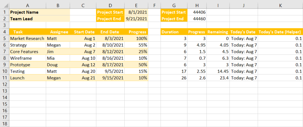
At the end of this stage, this is what you should run into:
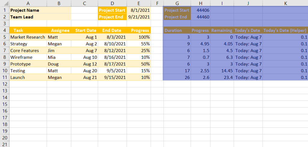
Here'south the breakup of the chart information highlighted in bluish to help you retrace the steps outlined beneath.
- Duration – The values in this column count the total number of days it takes to complete each task.
- Progress – This cavalcade converts the progress percent into the respective number of days spent on a given chore.
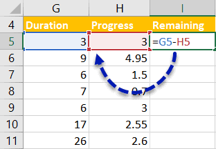
- Remaining – This column determines the remaining number of days it will take to complete a job based on the progress per centum points it takes to accomplish 100%.
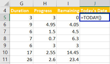
- Today's Date – This column pulls today's date using the TODAY function to position the electric current appointment line on the Gantt chart.
- Today'southward Date (Helper) – These helper values will exist used to create the reddish line illustrating today'due south appointment on the Gantt chart.
- Project Start & Project End – These values catechumen the project start date and end appointment in cells E1 and E2 into sequential serial numbers which we volition use to define the horizontal axis limits. For instance, the date "nine/21/2021" equals "44460" which indicates the number of days since January 1, 1900.
Whew, that was a lot of theory, so let's go cracking.
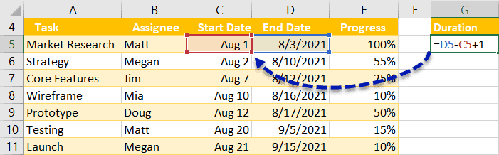
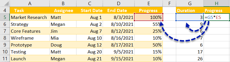
4. Start with populating column Duration (G4:G11). Create a column named "Duration" (G4), type "=D5-C5+1" into cell G5, and copy the formula down into cells G6:G11 using the fill handle.
The formula subtracts the task offset date (C5) from the job stop date (D5) and adds one day to come upwardly with the number of days it will accept to complete a given job.
v. Create a column named "Progress" (H4), enter "=G5*E5" into H5, and copy the formula down.
This formula picks the number of days information technology takes to consummate a task (G5) and uses the values in column Progress (E5) to calculate the progress on each task.
6. Ready some other column named "Remaining" (I4), type "=G5-H5" into I5, and re-create the formula into the remaining cells in the column (I6:I11).
7. Put together yet some other column called "Today'due south Date" (J4), blazon "=TODAY()" into J5, and copy the role into the remainder of the cells (J6:J11).
This elementary office dynamically returns today'due south date to aid Excel accurately display the current date on the Gantt chart.
Since the default date format just doesn't cut it for displaying the values on the chart, allow's spruce it upward a bit.
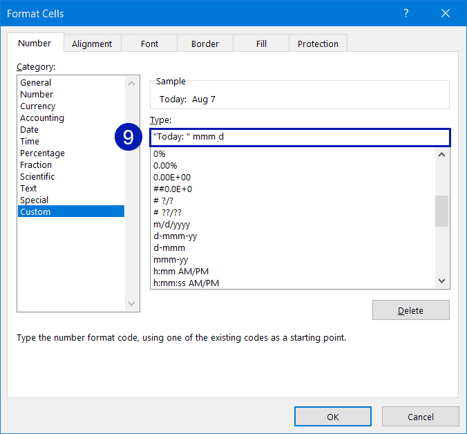
8. Highlight all the values in column Today's Engagement (J5:J11), correct-click on them, and cull "Format Cells."
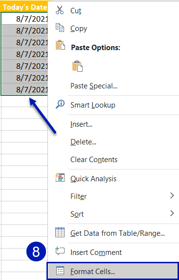
nine. In the dialog box that appears, choose the Custom choice for the Category, enter "Today:" mmm d (make certain you include the quotation marks around "Today:") into the "Type:" field, and click "OK."
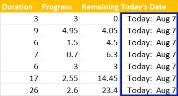
Once y'all accept done that, here'southward how that column should look:
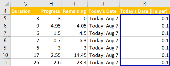
ten. Finally, create a column named "Today's Appointment (Helper)" (K4), enter "0.1" into K5, and re-create the value into the rest of the cells (K6:K11).
These values will make up a sparse vertical line to brandish the electric current date on the Gantt nautical chart.
Equally the last stride before we tin offset building out our Gantt graph, convert the projection start and terminate dates into the corresponding numeric code to come up with the values that will be used to set up the limits of the Gantt chart.
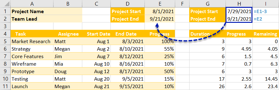
11. Duplicate the "Project Start" and "Project Terminate" labels (D1 and D2) into cells G1 and G2. Enter "=E1-iii" into H1. Type "=E2" into cell H2.
The value in cell H1 copies the project start engagement and subtracts three days from it to exit some infinite for the assignee labels on the chart and to prevent the chart elements from overlapping—y'all can tweak it however y'all see fit.
The value in prison cell H2 simply copies the project stop date.
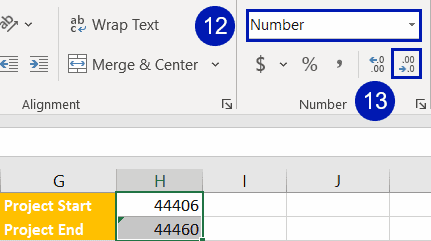
12. Select the values in cells H1:H2 and format the dates every bit "Numbers."
13. Hit the "Decrease Decimal" button twice to remove the decimal points.
By the terminate of this stage, here's how your worksheet should expect. Double-check everything simply in case and move on to the next footstep.
Step iii. Create a Stacked Column Nautical chart
I know, I know. You can't wait to jump into action. Well, allow'southward finally go to building out the Gantt nautical chart.
Right off the bat, lay down the foundation by creating a elementary stacked bar chart.
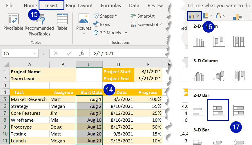
14. Highlight all the values in column Starting time Appointment (C5:C11).
15. Go to the Insert tab.
16. Choose "Insert Column or Bar Chart."
17. Select "Stacked Bar."
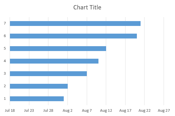
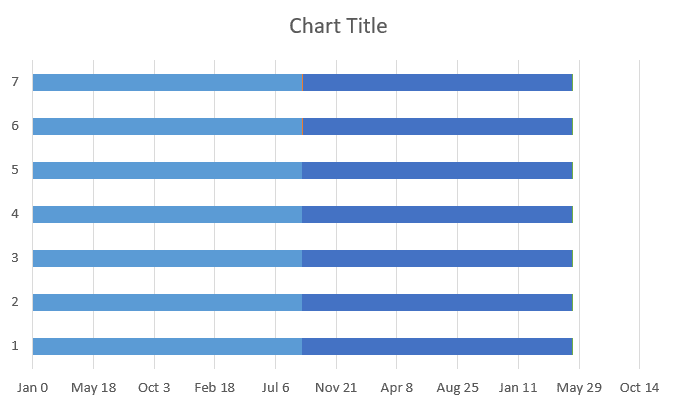
Magically, your stacked bar chart, the starting indicate of our g adventure, will appear.
Step 4. Add New Data Series
We haven't prepared all that chart information but for it to collect dust, so let'southward push all of that into the nautical chart plot.
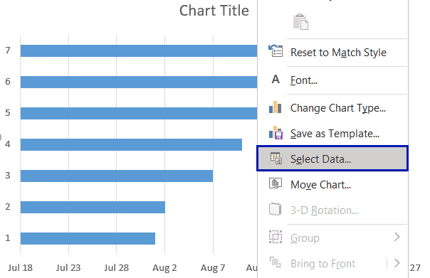
eighteen. Right-click on the chart plot and choose "Select Data."
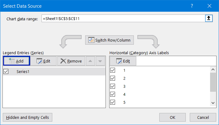
xix. In the Select Data Source dialog box, click the "Add" button.
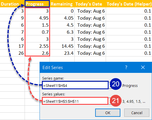
20. In the "Serial name" field, click the header row of cavalcade Progress (H4).
21. In the "Serial values" field, select all of the values in column Progress (H5:H11) and click "OK."
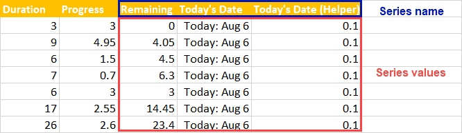
22. Rinse and repeat the same process to create Series "Remaining," Series "Today'south Appointment," and Series "Today'southward Date (Helper)" by following the exact same process outlined in steps #19–21.
At the end of this stage, order your data serial in the way shown on the screenshot below:
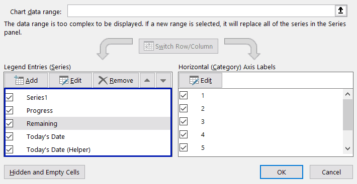
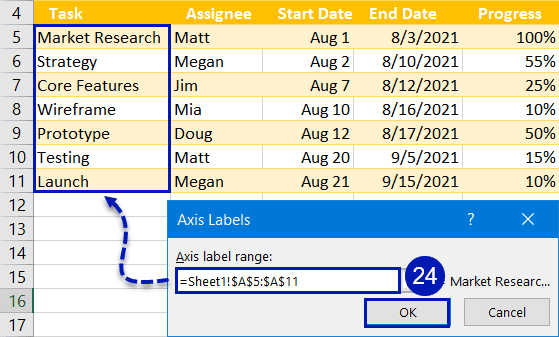
Hither's how your stacked bar chart should wait. Don't worry—we'll sort out this mess shortly.
Step v. Change the Vertical Axis (Add the Tasks)
Next finish: setting up the vertical centrality labels represented past the names of the tasks pulled from your original data table.
23. While notwithstanding in the Select Data Source dialog box, look under "Horizontal (Category) Axis Labels" and click "Edit."
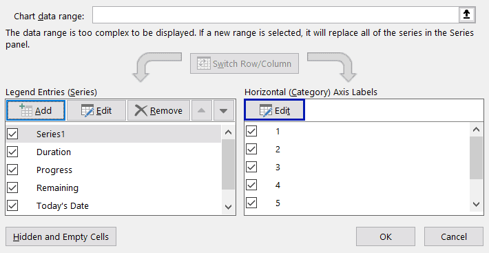
24. For the "Axis label range" field, highlight all of the tasks from your table (A5:A11) and click "OK."
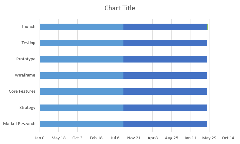
25. Save the changes yous made past clicking "OK" twice to close out of the dialog box. At this point, your chart should look something like this:
Footstep half-dozen. Contrary the Category Order
As you may take noticed, something is off with the vertical axis. Let'south fix it up quickly with merely a few pocket-size tweaks.
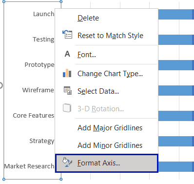
26. Right-click on the vertical centrality and choose "Format Centrality."
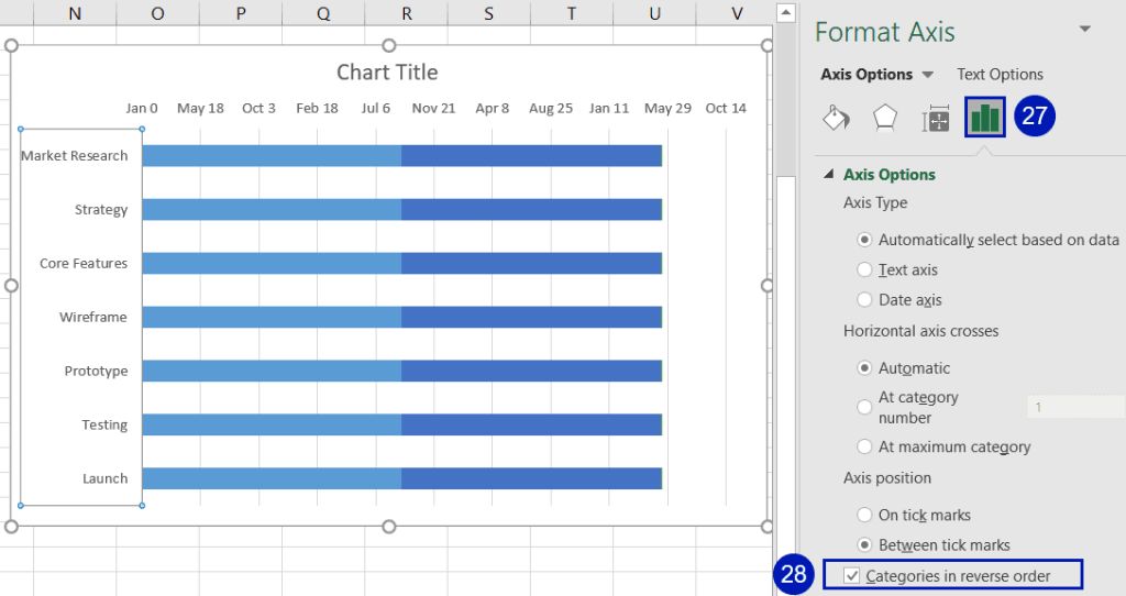
27. Switch over to the Axis Options tab.
28. Under "Axis Position," check the box next to "Categories in reverse social club" to plough the chart upside downwardly and put everything back in its place.
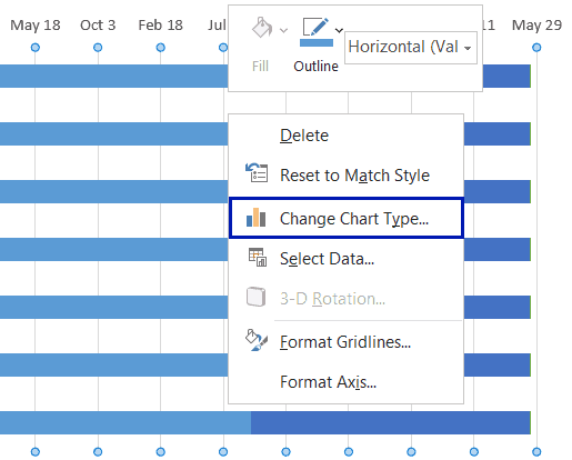
29. After that, right-click on the nautical chart area and cull "Change Chart Blazon."
30. In the Combo tab, set the "Nautical chart Type" value to "Stacked Bar" for every single data serial.
31. Check the "Secondary Axis" boxes for Series "Today's Date" and Series "Today's Date (Helper)" and click "OK" to close the dialog box.
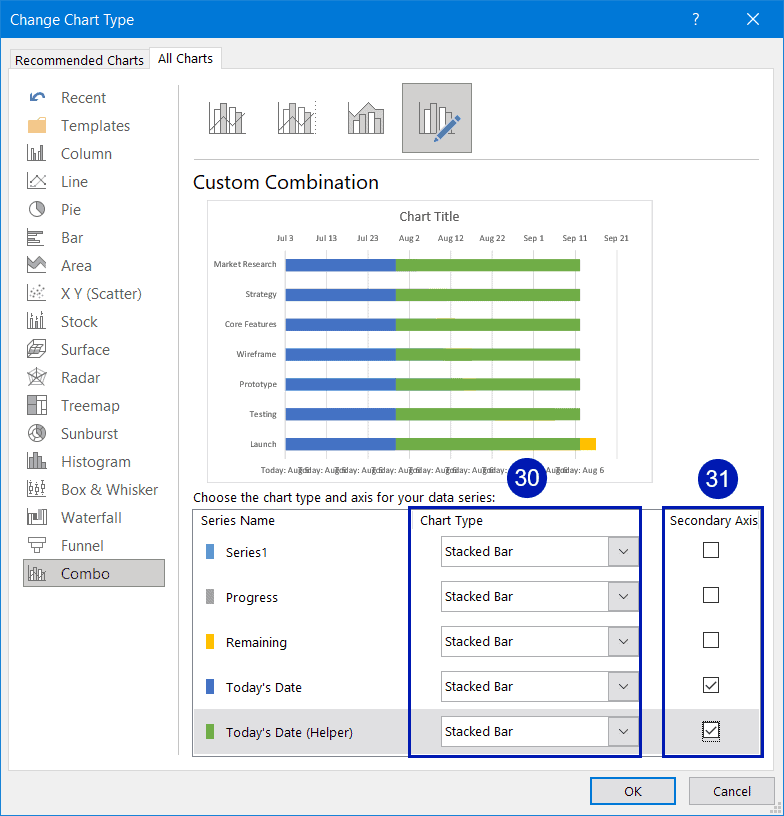
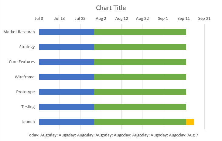
Having done that, here'southward what your nautical chart should look like:
Pace seven. Create a Gantt Chart
It'due south fourth dimension to put all the pieces of our puzzle together and transform the mess that we currently take into a powerful Gantt chart.
To do that, we merely demand to friction match the bound values of both the axes.
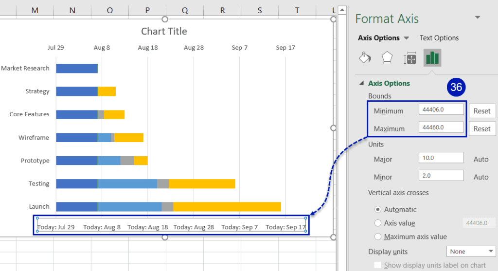
32. Correct-click on the master axis and click "Format Centrality."
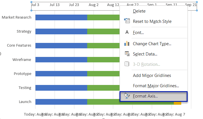
33. Striking the "Axis Options" push button.
34. Nether "Bounds," set the "Minimum" value to the converted value of the project start engagement (H1).
35. Change the "Maximum" value to the converted value of the projection end date (H2).
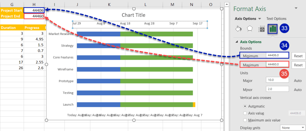
36. Repeat the same process outlined in steps #34–35 for the secondary centrality and watch your chart magically transform. In one case at that place, delete the secondary axis (the one highlighted on the screenshot beneath) by pressing the Delete cardinal.
Footstep 8. Clean Upwards the Axes
Permit'south clean upwardly the axes a bit to start seeing the get-go signs of our lovely Gantt chart.
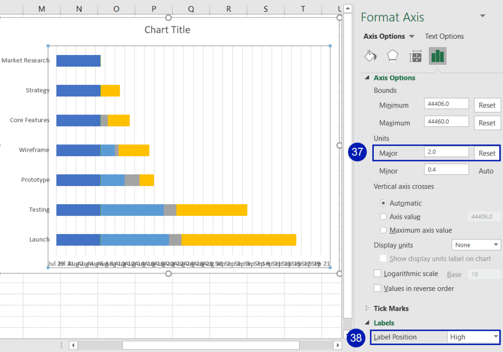
37. Switch back to the main axis. In the same Axis Options tab, under "Units," fix the "Major" value to "2." This value determines the intervals of the days on the primary axis scale, so you can tweak it even so you want.
38. Alter "Characterization Position" to "High" to re-position the axis position.
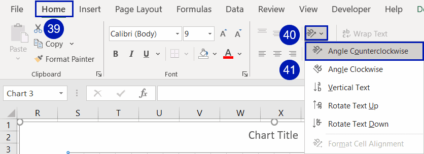
39. Without de-selecting the main axis, slightly rotate the axis labels for everything to fall into its place. To starting time with, click the Dwelling house tab.
forty. Hit the "Orientation" button.
41. Select "Bending Counterclockwise."
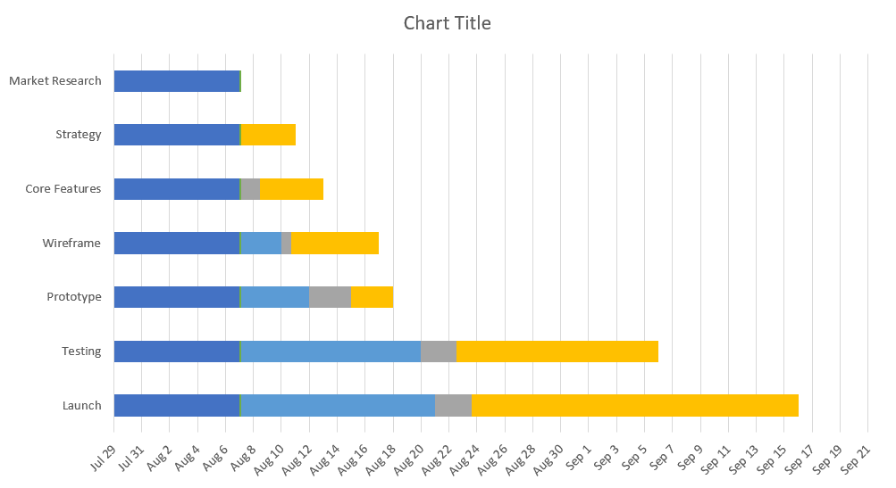
Let's have a quick peek at our Gantt chart. Here's how it should wait now:
Step 9. Gear up the Today Line
42. Right-click on Series "Today's Date" represented by the dark blue horizontal bars (all of the aforementioned size) and click "Format Data Series."
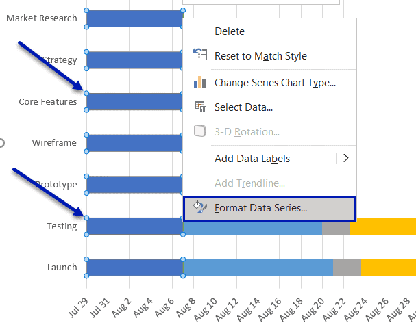
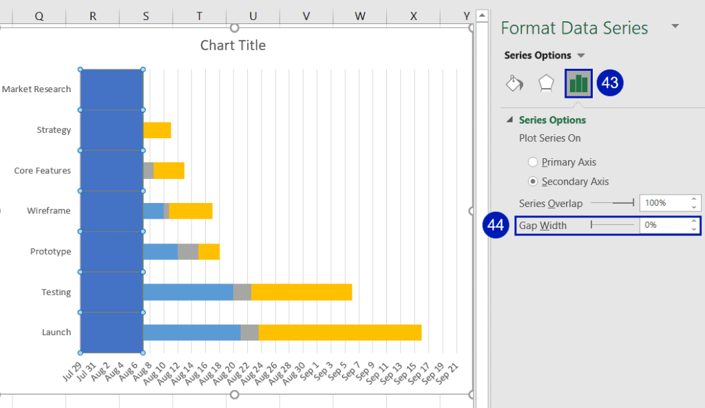
43. In the Format Data Series job pane, go to the Series Options tab.
44. Change the "Gap Width" value to "0%."
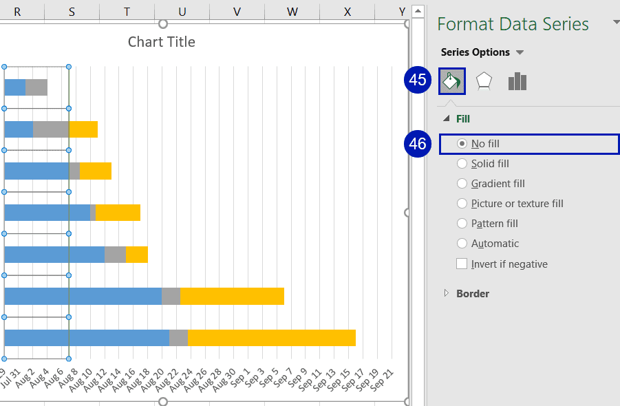
45. Switch to the Fill & Line tab.
46. Under "Fill," cull "No fill" to make the data serial transparent.
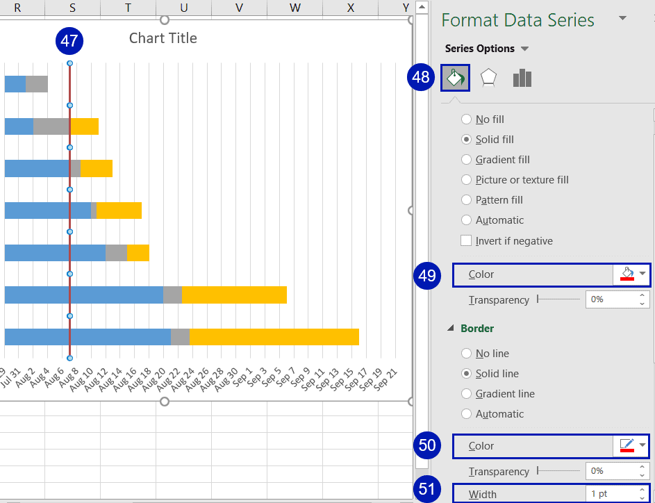
47. Jump to Series "Today'due south Data (Helper)" without closing the tab.
48. Click the Fill & Line icon.
49. Change the fill color to red.
l. Set the border fill color to ruby.
51. Under "Edge," set the "Width" value to "one pt."
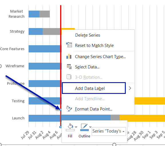
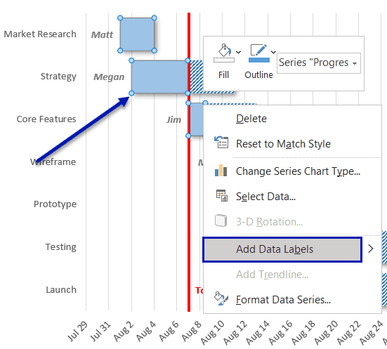
52. If you want to add the custom data label that we previously prepare up, double-click at the bottom of the vertical red line, right-click on it, and select "Add Data Label."
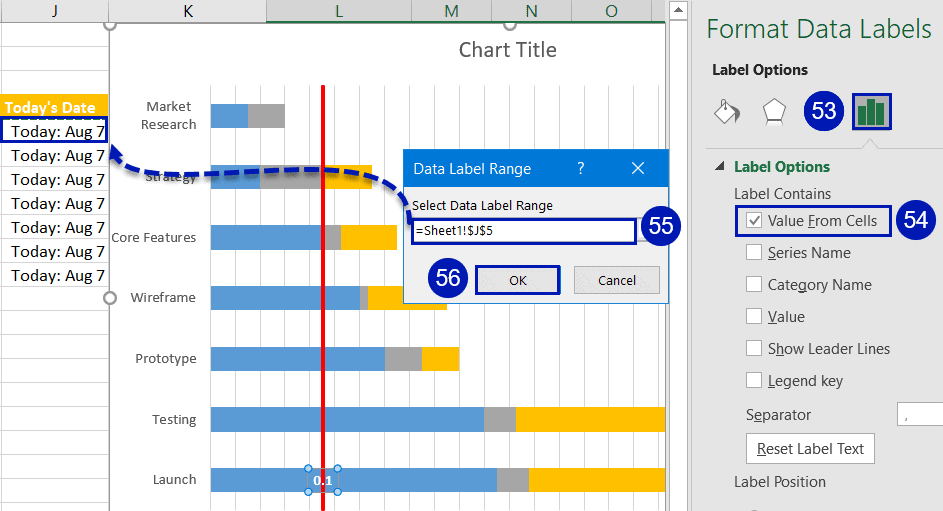
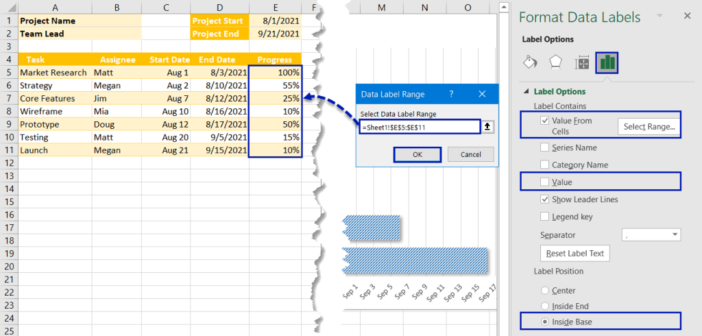
53. Select the Data Label and click the "Characterization Options" button in the Format Data Labels pane.
54. Check the "Value From Cells" box.
55. For "Select Information Label Range," select any value in column Today'due south Date to set up a custom data label.
56. Click "OK" to apply changes.
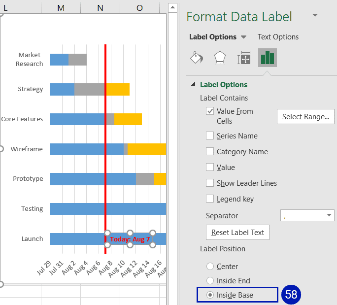
57. In the same tab, double-click the "Value" checkbox to remove the default data labels. (This will add them then take them abroad once more.)
58. Finally, alter the label color to red (Habitation > Font > Font Color) and make the characterization bold (Home > Bold). In the Label Options tab, under "Label Position," cull "Inside Base of operations."
Stride 10. Gear up the Task Bars
Earlier nosotros call it a mean solar day, all nosotros need to do is set upward the job bars to help your team keep track of whether y'all're ahead of or behind schedule.
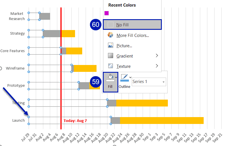
59. Hibernate the bars supporting the Gantt chart. Right-click on the helper Series "Start Date" holding the task bars together and select "Make full."
60. In the carte that appears, choose "No Fill."
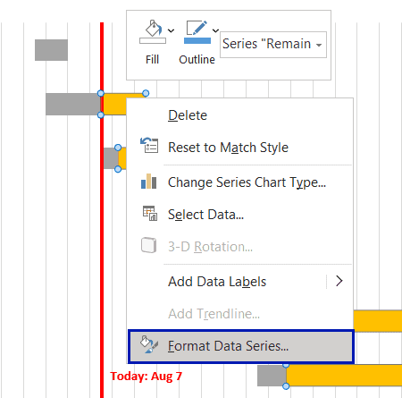
61. Correct-click on Series "Remaining," represented by the orangish bars, and cull "Format Information Series."
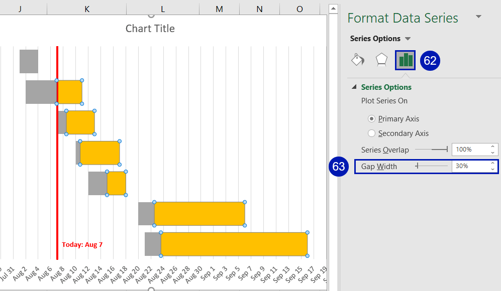
62. Click the "Series Options" icon.
63. Change the "Gap Width" value to "30%."
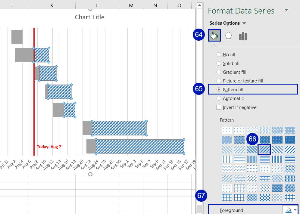
64. Navigate to the Fill & Line tab.
65. Nether "Fill," select "Design make full."
66. Pick "Diagonal stripes: Nighttime upwardly" from the options that appear.
67. Alter the "Foreground" to night blueish.
Switch to Series "Progress," represented by the grayness bars, and recolor them to make the color scheme consequent:
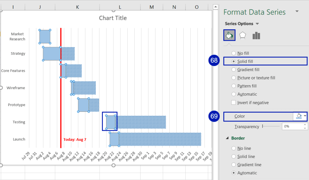
68. In the Fill & Line tab, under "Fill up," select "Solid make full."
69. Next to "Color," click the "Fill Color" icon and change the color of the data serial to light bluish.
seventy. In the Format Information Series task pane, get to the Effects tab.
71. Click the "Shadow" button.
72. Under "Presets," select the dropdown to the right. In the menu that pops up, under "Outer," cull "Offset: Lesser Right."

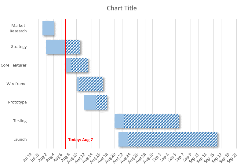
73. Echo the same stride for Series "Remaining." At the end of this stride, your Gantt chart should look like this:
Stride xi. Add the Assignee & Progress Labels
Technically, you can stop right there. Merely alternatively, we can make our Gantt chart a lot more than descriptive and informative past adding the data labels illustrating the corresponding assignee and progress for every unmarried task.
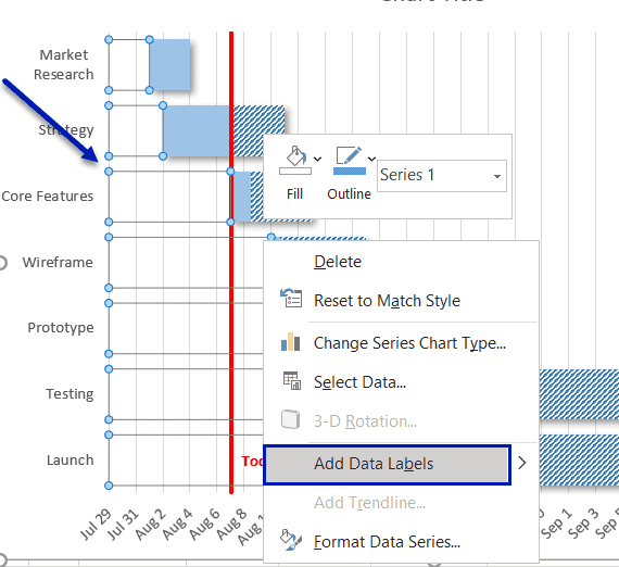
74. Right-click the subconscious Series "Date Start" holding the task bars together and choose "Add Data Labels."
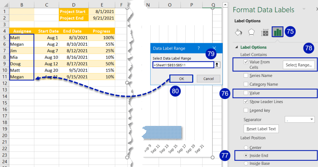
75. Select the labels and go to the Label Option tab.
76. Uncheck the "Value" box.
77. Nether "Label Position," select "Inside End."
78. Under "Label Contains," click "Value From Cells."
79. In the Data Characterization Range dialog box, select all the values in column Assignee (B5:B11).
80. Click "OK" to apply changes.
Modify the font size and color for the labels to fit them meliorate on the chart—and take a look at the results of all your hard work:
81. Correct-click on Series "Progress," represented past the light bluish vertical bars, and click "Add Data Labels."
82. Adjust the progress information labels by repeating steps #75–lxxx . In this instance, however, set up the "Label Position" value to "Inside Base of operations" and apply the Progress data from E5:E11 when you lot set the "Value From Cells."
All yous have left is to bandbox upwards the progress information labels to make them stand out.
83. Modify the characterization font color to white.
84. Change the label groundwork color to black.
85. Apply the bold and italic font formatting.
86. Alter the font size to "8."
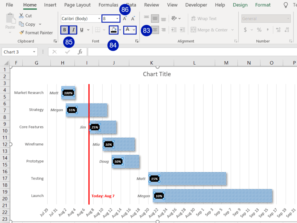
Finally, change the chart title, and you lot're all set!
Short on Time? Catch This Free Excel Gantt Nautical chart Template (with Stride-by-pace Setup Instructions)
Download Gratis Gantt Chart Template
As you can see from all of the steps covered higher up, building this Gantt chart template takes quite a scrap of time.
So if you're short on time, grab a free Gantt nautical chart template by clicking the link above and follow simple instructions to adjust the template to your actual data.
Let'southward zoom out and take a look at the entire template.
On the screenshot beneath, the merely columns and values you need to alter to get upwardly and running are highlighted in blue while the rest gets adjusted automatically based on your actual values.
Here's the breakdown of the values that you need to conform:
Columns A, B, C, D, Eastward – these columns are pretty self-explanatory. Use them to name your tasks, create assignees, specify the first and end appointment of every task, and keep rails of your progress.
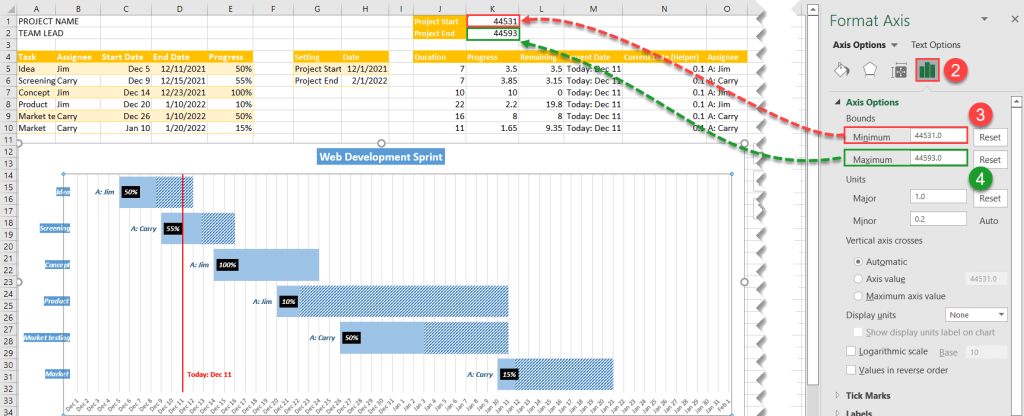
Column G and H – These are the just columns that are a bit trickier. The values in cells H5 (12/ane/2021) and H6 (two/1/2022) are getting copied into cells K1 (44531) and K2 (44593). One time in that location, they converted into the corresponding numerical values – since all dates in Excel are stored as numbers.
These values define the starting time and end of the horizontal axis. That being said, you need to tweak the "Project Showtime" (H5) and "Project End" (H6) values in a way that prevents the assignee labels from overlapping the vertical centrality of your Gantt chart.
Once there, you demand to accommodate your horizontal axis.
1. Correct-click on the horizontal centrality and select "Format Centrality."
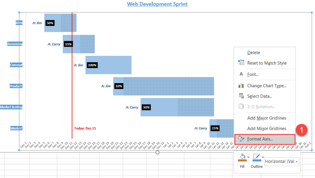
two. Hit the "Axis Options" icon.
iii. Under "Bounds," set the "Minimum" value to the value in jail cell E1 (44531).
4. Under "Bounds," change the "Maximum" value to the value in cell E2 (44593).
Once at that place, your chart is all set and prepare to go.
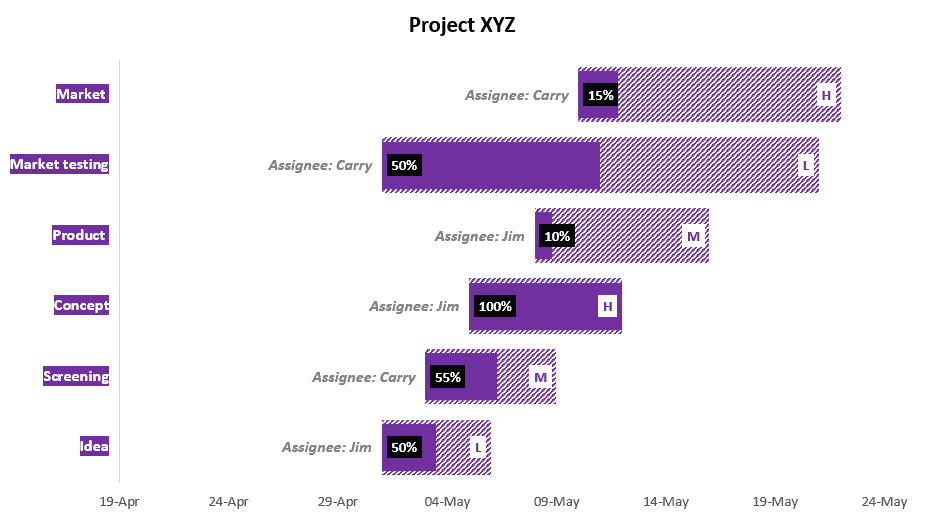
Free Excel Gantt Chart Template #2 – Simplified Version
Download Free Gantt Chart Template #2
Are you looking for something simple nonetheless professionally-looking? We've got you covered! This simplified version of our Gantt nautical chart template has simply everything you demand to manage your projects effectively.
The setup process takes less than 2 minutes. So, let's dive right in.
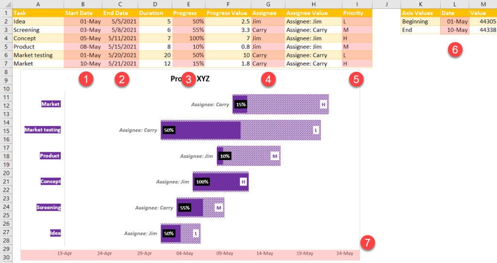
To go up and running, you demand to modify seven elements of the template while the residual is adjusted automatically:
- Column Start Date – this column stores all the values corresponding with the start engagement of each of the tasks.
- Cavalcade End Appointment – this cavalcade contains all the values corresponding with the end of each of the tasks.
- Column Progress – Use this column to go along track of your progress.
- Column Assignee – Apply this column to assign team members to each of your tasks.
- Column Priority – This helper column helps teams prioritize their efforts for better operation.
- Column Appointment – These two values generate the nautical chart axis values for cavalcade M that you volition need to employ to accommodate the axis based on your dates, helping you forestall your nautical chart from getting messy.
Hither'southward how these values are generated: The underlying formula subtracts a few days from the get-go appointment of your first chore and adds a few days to the end of your terminal task to prevent the labels from overlapping. Once there, The values are copied into cavalcade M and get converted into numbers.
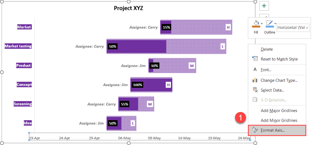
- The Horizontal Centrality – Finally, y'all need to conform the horizontal axis. This part is a bit tricky, so let'due south cover it in greater detail.
1. Select the nautical chart centrality, right-click on it, and choose "Format Axis."
2. Once the Format Axis task pane appears, click "Axis Options."
3. Set the "Minimum Bounds" to the value in prison cell M1 (44305).
iv. Set the "Maximum Bounds" to the value in prison cell M2 (44338).
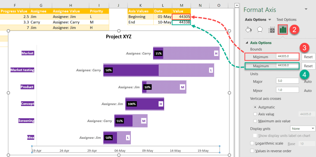
Ta-da! You're all set. Your lovely Gantt nautical chart is gear up to become.

How To Use Excel Chart Templates 2021,
Source: https://spreadsheetdaddy.com/excel/gantt-chart
Posted by: hurleyalubly.blogspot.com
0 Response to "How To Use Excel Chart Templates 2021"
Post a Comment